
# Comments inside an R cell begin with #, just as they do in an R script.
x <- c(2, 4, 6, 8, 10)
mean(x)[1] 6Write reproducible documents with R
This is the starting point for working with Quarto. It focuses on the small set of ideas needed to create a clear, reproducible document without assuming previous experience.
Already comfortable with the basics? Continue to the Quarto reference for reusable commands and patterns, or copy the report template when starting a new analysis.
Quarto is a way to write reproducible reports that keep your explanations, R code, figures, tables, and results together. Quarto files use the .qmd extension and can produce HTML, PDF, Word, presentations, websites, and books.
Most of the file is ordinary text. R code only runs when it is placed inside an R code cell.
Install Quarto, R, and RStudio. In RStudio:
RStudio creates a sample document. You can delete the example content below the YAML header and start writing your own report.
Do not delete the opening and closing --- lines. They define the document header.
The YAML header controls the title, author, date, output format, and document options.
---
title: "My Quarto report"       # Document title
author: "Your name"             # Author name
date: today                     # Current date
toc: true                       # Add a table of contents
format:
  html:
    theme: flatly               # HTML appearance
    embed-resources: true       # Create one self-contained HTML file
execute:
  warning: false                # Hide warnings in the final document
  message: false                # Hide package messages
---
YAML indentation matters. Use spaces, keep nested options aligned, and do not use tabs.
Add # characters at the beginning of a line to create sections. More # characters create lower-level headings.
# Main section

## Subsection

### Smaller subsection

#### Fourth-level heading

##### Fifth-level heading

###### Sixth-level heading
Use headings in order. A document normally starts with #, then uses ## and ### to organize related content.
Code cells are the places where you write executable R code. Everything outside a code cell is treated as text.
There are three common ways to insert an R cell:
```{r} at the beginning and ``` at the end.# Comments inside an R cell begin with #, just as they do in an R script.
x <- c(2, 4, 6, 8, 10)
mean(x)[1] 6To run code without rendering the entire document:
Objects created in one cell are available to later cells during the same session and render.
Cell options begin with #| and apply only to that cell.
summary(mtcars$mpg) Min. 1st Qu. Median Mean 3rd Qu. Max.
10.40 15.43 19.20 20.09 22.80 33.90 | Option | Effect |
|---|---|
#| echo: false |
Run the code but hide it |
#| output: false |
Hide printed output |
#| include: false |
Hide both code and output |
#| eval: false |
Display code without running it |
#| warning: false |
Hide warnings |
#| fig-width: 7 |
Set figure width in inches |
Use inline R code when a value should update automatically:
The mean fuel economy is 20.1 miles per gallon.The rendered result is: the mean fuel economy is 20.1 miles per gallon.
Quarto uses Markdown for ordinary writing.
**Bold text**

*Italic text*

`code or an object name`

- an unordered list
- another item

1. the first step
2. the second step
The formatting appears as bold text, italic text, and inline code in the rendered document.
Add a link with descriptive text followed by the URL:
[RStudio and Posit cheat sheets](https://posit.co/resources/cheatsheets/)Add an image with similar syntax, but place ! at the beginning:
The image can be a local file or a web URL. Local images should be stored inside the project and referenced with a relative path.

Use knitr::kable() for a simple table:
car_summary <- aggregate(mpg ~ cyl, data = mtcars, FUN = mean)
knitr::kable(
  car_summary,
  digits = 1,
  col.names = c("Cylinders", "Mean MPG")
)| Cylinders | Mean MPG |
|---|---|
| 4 | 26.7 |
| 6 | 19.7 |
| 8 | 15.1 |
R graphics are inserted at the position of the code cell:
plot(
  mtcars$wt,
  mtcars$mpg,
  pch = 19,
  col = "#2878B5",
  xlab = "Weight (1,000 lb)",
  ylab = "Fuel economy (mpg)"
)
abline(lm(mpg ~ wt, data = mtcars), col = "#C82423", lwd = 2)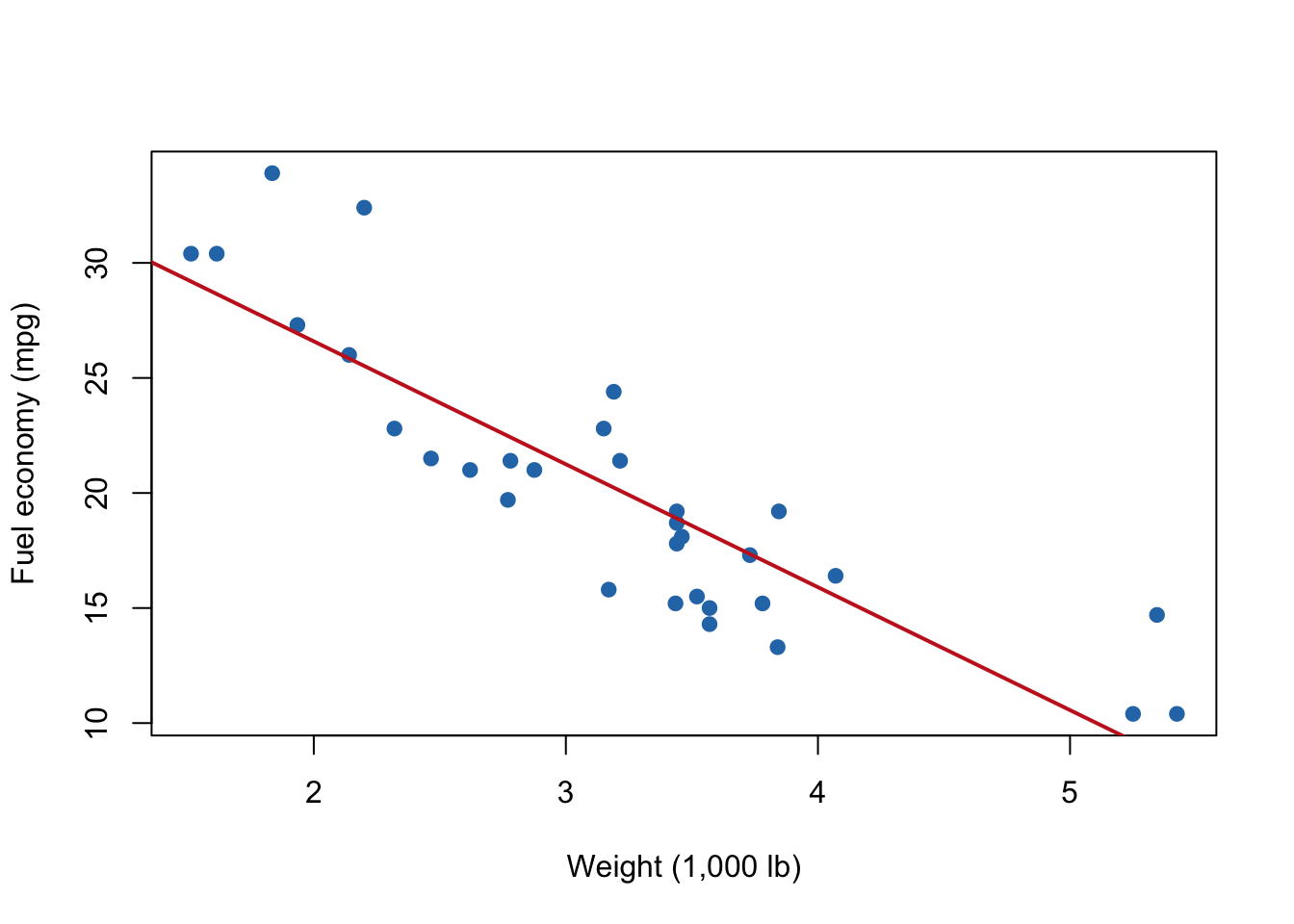
Labels beginning with tbl- or fig- can be referenced in the text. For example, Table 1 summarizes the cars and Figure 1 displays the relationship between weight and fuel economy.
Create a footnote with [^1] in the text and define it elsewhere in the document:
Quarto supports footnotes.[^1]

[^1]: This is the footnote text.
For academic citations, add a BibTeX file to the header:
bibliography: references.bibThen cite an entry with [@citation-key]. Quarto creates the reference list automatically.
Click Render at the top of the RStudio editor. Quarto runs the code from top to bottom and creates the requested output.
You can also render from a terminal:
quarto render index.qmdChange the YAML to select another format:
format: htmlformat: docxformat: pdfPDF output requires a TeX installation. HTML is usually the easiest format for a first document.
Before sharing, restart R and render again. This confirms that the document loads every package, creates every object, and does not depend on items left in the interactive environment.